Introduction
In bmcmc, we fit a statistical model specified by a set of
parameters \(\theta\) to some data \(D\). Using
MCMCM we sample the posterior \(p(\theta|D)\). A
statistical model is specified by defining a subclass derived
from the parent class bmcmc.Model and
the user has to write 3 methods for his subclass. We
show this with a simple example.
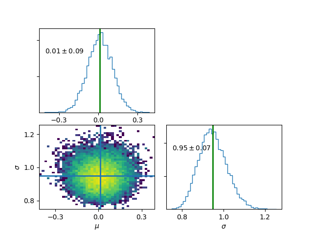
Fitting a Gaussian distribution
A Gaussian or a normal distribution is given by \(\mathcal{N}(x|\mu,\sigma^2)=\frac{1}{\sqrt{2 \pi}\sigma}\exp\left[-\frac{(x-\mu)^2}{2\sigma^2}\right]\) and we fit this to an array of values representing samples from a one dimensional distribution.:
import bmcmc
import scipy.stats

class gauss1(bmcmc.Model):
    def set_descr(self):
        # setup descriptor
        # self.descr[varname]=[type, value, sigma,     latexname, min_val, max_val]
        self.descr['mu']     =['l0',   0.0,   1.0,      r'$\mu$',    -500,   500.0]
        self.descr['sigma']  =['l0',   1.0,   1.0,   r'$\sigma$',  1e-10,      1e3]

    def set_args(self):
        # setup data points
        # Use self.args and self.eargs to define your variables.
        # During sampling, the code will pass self.args as an argument to lnfunc.
        np.random.seed(11)
        self.args['x']=np.random.normal(loc=0.0,scale=1.0,size=self.eargs['dsize'])

    def lnfunc(self,args):
        # define the function which needs to be sampled (log posterior)
        # Do not use self.args in this function. You can use self.eargs.
        return scipy.stats.norm.logpdf(args['x'],loc=args['mu'],scale=args['sigma'])
Create an object. The bmcmc.Model
accepts a keyword argument named eargs which should be a
dictionary. In the class, it is available as self.eargs.
Through this keyword one can pass any external information
to the class.
>>> mymodel=gauss1(eargs={'dsize':50})
Run the sampler for two free parameters, for 50000 iterations, printing summary every 10000 iterations.
>>> mymodel.sample(['mu','sigma'],50000,ptime=10000)
Print final results, discarding first 10000 iterations
>>> mymodel.info(burn=5000)
no             name         mean      stddev [         16%,          50%,          84%]
Level-0
0               mu    0.0121747    0.0955931 [  -0.0818376,    0.0127852,     0.106895]
1            sigma     0.948579    0.0680425 [    0.880681,     0.944834,      1.01692]
Plot final results , discarding first 5000 iterations
>>> mymodel.plot(burn=5000)
Print chain values for a few given parameters
>>> print mymodel.chain['mu']
>>> print mymodel.chain['sigma']
To print final results as a latex table, discarding the first 5000 iterations.
>>> mymodel.info(burn=5000,latex=True)
\begin{tabular} { l  c}
Parameter &  16 and 84 \% limits\\
\hline
$\mu$ & $0.01^{+0.09}_{-0.09}$ \\
$\sigma$ & $0.95^{+0.07}_{-0.07}$ \\
\hline
\end{tabular}
Plot final results for specific parameters
>>> mymodel.plot(keys=['mu','sigma'],burn=1000)
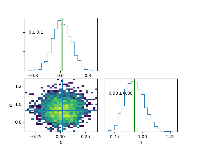
Bayesian hierarchical model (BHM).
We again consider the example of fitting a Gaussian distribution to some observed data. This time the observed data \(x\) has uncertainty \(\sigma_x\) associated with it. The true values \(x_t\) is unknown which we estimate alongside the parameters of the Gaussian distribution \(\theta=\{ \mu,\sigma\}\). The posterior is given by
The Metropolis-Within-Gibbs scheme is used for sampling the posterior. While \((\mu,\sigma)\) are level-0 parameters, \(x_t\) is at level-1. This makes the model hierarchical. A wide variety of real world problems fall into this category. This method provides a way to marginalize over observational uncertainties via sampling but rather than doing any integration. Missing or hidden variables can also be marginalized in a similar fashion.
class gauss2(bmcmc.Model):
    def set_descr(self):
        # setup descriptor
        self.descr['mu']     =['l0',0.0,1.0,r'$\mu$'   ,-500,500.0]
        self.descr['sigma']  =['l0',1.0,1.0,r'$\sigma$',1e-10,1e3]
        self.descr['xt']     =['l1',0.0,1.0,r'$x_t$'   ,-500.0,500.0]

    def set_args(self):
        # setup data points
        np.random.seed(11)
        # generate true coordinates of data points
        self.args['x']=np.random.normal(loc=self.eargs['mu'],scale=self.eargs['sigma'],size=self.eargs['dsize'])
        # add observational uncertainty to each data point
        self.args['sigma_x']=np.zeros(self.args['x'].size,dtype=np.float64)+0.5
        self.args['x']=np.random.normal(loc=self.args['x'],scale=self.args['sigma_x'],size=self.eargs['dsize'])

    def lnfunc(self,args):
        # log posterior
        temp1=scipy.stats.norm.logpdf(args['xt'],loc=args['mu'],scale=args['sigma'])
        temp2=scipy.stats.norm.logpdf(args['x'],loc=args['xt'],scale=args['sigma_x'])
        return temp1+temp2
Create an object and run the sampler.
>>> mymodel=gauss2(eargs={'dsize':100,'mu':1.0,'sigma':2.0})
>>> mymodel.sample(['mu','sigma','xt'],50000,ptime=1000)
Note, for level-1 parameters,
each data point has its own value for the parameter.
Rather than storing the full chain, only mean
and standard-deviation for each data point are stored and
made available. These can be accessed as follows.
To print mean value of xt for each data point
>>> print mymodel.mu['xt']
[ 1.68764301 -0.191843  ...,  0.80656432  0.47805343]
To print stddev of xt for each data point
>>> print mymodel.sigma['xt']
[ 0.44846551  0.43683076  ...,  0.44343331  0.44246093]
Print final results. For level-1 parameters the printed values are just average taken over all data points.
>>> mymodel.info()
no            name         mean       stddev [         16%,          50%,          84%]
Level-0
0               mu    0.0141504     0.106783 [  -0.0919234,     0.013786,     0.119224]
1            sigma     0.929101    0.0875563 [    0.842694,     0.923683,      1.01629]
Level-1
0               xt    0.0132397     0.441688
>>> mymodel.plot(burn=5000)
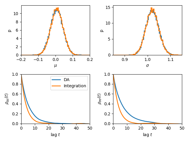
Data Augmentation
We can also estimate \(\theta=\{\mu,\sigma\}\) by explicitly integrating out the \(x_t\). The posterior is given by
Autocorrelation analysis shows that explcit integration reduces the correlation length. However, not all functions can be easily integrated.
class gauss3(bmcmc.Model):
  def set_descr(self):
      # setup descriptor
      self.descr['mu']     =['l0',0.0,1.0,r'$\mu$ ',-500,500.0]
      self.descr['sigma']  =['l0',1.0,1.0,r'$\sigma$ ',1e-10,1e3]

  def set_args(self):
      # setup data points
      np.random.seed(11)
      # generate true coordinates of data points
      self.args['x']=np.random.normal(loc=self.eargs['mu'],scale=self.eargs['sigma'],size=self.eargs['dsize'])
      # add observational uncertainty to each data point
      self.args['sigma_x']=np.zeros(self.args['x'].size,dtype=np.float64)+0.5
      self.args['x']=np.random.normal(loc=self.args['x'],scale=self.args['sigma_x'],size=self.eargs['dsize'])

  def lnfunc(self,args):
      # log posterior, xt has been integrated out
      sigma=np.sqrt(args['sigma']*args['sigma']+args['sigma_x']*args['sigma_x'])
      temp=scipy.stats.norm.logpdf(args['x'],loc=args['mu'],scale=sigma)
      return temp

 # Data augmentation, making use of Hierarchical modelling
 # marginalization using sampling.
 m2=gauss2(eargs={'dsize':1000,'mu':0.0,'sigma':1.0})
 m2.sample(['mu','sigma','xt'],100000,ptime=10000)
 # Marginalization using direct integration
 m3=gauss3(eargs={'dsize':1000,'mu':0.0,'sigma':1.0})
 m3.sample(['mu','sigma'],100000,ptime=10000)

 plt.subplot(2,2,1)
 plt.hist(m2.chain['mu'],range=[-0.2,0.2],bins=100,normed=True,histtype='step',lw=2.0)
 plt.hist(m3.chain['mu'],range=[-0.2,0.2],bins=100,normed=True,histtype='step',lw=2.0)
 plt.ylabel('p')
 plt.xlabel(r'$\mu$')
 plt.xlim([-0.2,0.2])
 plt.xticks([-0.2,-0.1,0.0,0.1,0.2])

 plt.subplot(2,2,2)
 plt.hist(m2.chain['sigma'],range=[0.85,1.15],bins=100,normed=True,histtype='step',lw=2.0)
 plt.hist(m3.chain['sigma'],range=[0.85,1.15],bins=100,normed=True,histtype='step',lw=2.0)
 plt.ylabel('p')
 plt.xlabel(r'$\sigma$')
 plt.xlim([0.85,1.15])
 plt.xticks([0.9,1.0,1.1])

 plt.subplot(2,2,3)
 nsize=50
 plt.plot(np.arange(nsize),bmcmc.autocorr(m2.chain['mu'])[0:nsize],label='DA',lw=2.0)
 plt.plot(np.arange(nsize),bmcmc.autocorr(m3.chain['mu'])[0:nsize],label='Integration',lw=2.0)
 plt.ylabel(r'$\rho_{\mu \mu}(t)$')
 plt.xlabel(r'lag $t$')
 plt.legend()
 plt.axis([0,50,0,1])

 plt.subplot(2,2,4)
 plt.plot(np.arange(nsize),bmcmc.autocorr(m2.chain['sigma'])[0:nsize],lw=2.0)
 plt.plot(np.arange(nsize),bmcmc.autocorr(m3.chain['sigma'])[0:nsize],lw=2.0)
 plt.ylabel(r'$\rho_{\sigma \sigma}(t)$')
 plt.xlabel(r'lag $t$')
 plt.axis([0,50,0,1])
 plt.tight_layout()
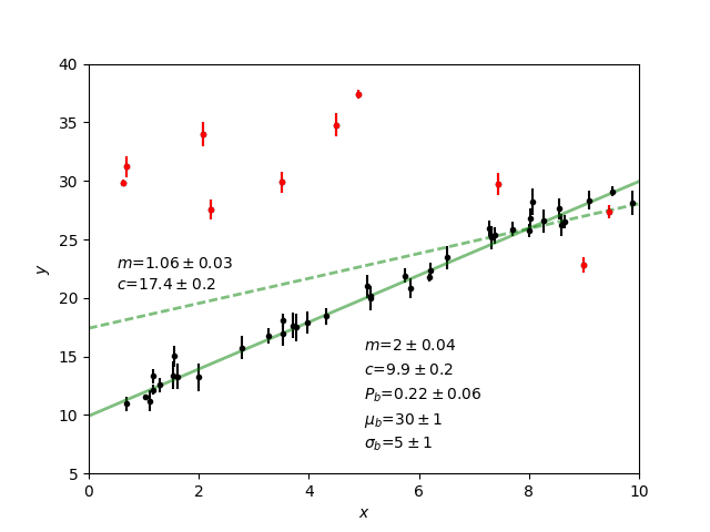
Fitting a straight line with outliers
We discuss the case of fitting a straight line to some data points \(D=\{(x_1,y_1),(x_2,y_2)...(x_N,y_N)\}\). The straight line model to decribe the points is
The background model to take the outliers into account is
The full model to describe the data is
The methods in the derived class for implementing the straight line model are as follows.
class stlineb(bmcmc.Model):
  def set_descr(self):
      # setup descriptor
      self.descr['m']      =['l0', 1.0, 0.2,'$m$',        -1e10,1e10]
      self.descr['c']      =['l0',10.0, 1.0,'$c$',        -1e10,1e10]
      self.descr['mu_b']   =['l0', 1.0, 1.0,'$\mu_b$',    -1e10,1e10]
      self.descr['sigma_b']=['l0', 1.0, 1.0,'$\sigma_b$', 1e-10,1e10]
      self.descr['p_b']    =['l0',0.1,0.01,'$P_b$',      1e-10,0.999]

  def set_args(self):
      # setup data points
      np.random.seed(11)
      self.args['x']=0.5+np.random.ranf(self.eargs['dsize'])*9.5
      self.args['sigma_y']=0.25+np.random.ranf(self.eargs['dsize'])
      self.args['y']=np.random.normal(self.args['x']*2+10,self.args['sigma_y'])
      # add outliers
      self.ind=np.array([0,2,4,6,8,10,12,14,16,18])
      self.args['y'][self.ind]=np.random.normal(30,5,self.ind.size)
      self.args['y'][self.ind]=self.args['y'][self.ind]+np.random.normal(0.0,self.args['sigma_y'][self.ind])

  def lnfunc(self,args):
      # log posterior
      if self.eargs['outliers'] == False:
          temp1=(args['y']-(self.args['m']*self.args['x']+self.args['c']))/args['sigma_y']
          return -0.5*(temp1*temp1)-np.log(np.sqrt(2*np.pi)*args['sigma_y'])
      else:
          temp11=scipy.stats.norm.pdf(args['y'],loc=(self.args['m']*self.args['x']+self.args['c']),scale=args['sigma_y'])
          sigma_b=np.sqrt(np.square(args['sigma_y'])+np.square(args['sigma_b']))
          temp22=scipy.stats.norm.pdf(args['y'],loc=self.args['mu_b'],scale=sigma_b)
          return np.log((1-args['p_b'])*temp11+args['p_b']*temp22)

  def myplot(self,chain):
     # optional method for plotting
     # plot best fit line corrsponding to chain of this model
      plt.clf()
      x = np.linspace(0,10)
      burn=self.chain['m'].size/2
      vals=self.best_fit(burn=burn)
      plt.errorbar(self.args['x'], self.args['y'], yerr=self.args['sigma_y'], fmt=".k")
      plt.errorbar(self.args['x'][self.ind], self.args['y'][self.ind], yerr=self.args['sigma_y'][self.ind], fmt=".r")
      plt.plot(x,vals[0]*x+vals[1], color="g", lw=2, alpha=0.5)
      for i,key in enumerate(self.names0):
          print key
          plt.text(0.5,0.3-i*0.06,self.descr[key][3]+'='+bmcmc.stat_text(self.chain[key][burn:]),transform=plt.gca().transAxes)

     # plot best fit line corrsponding to some other chain
      vals1=[]
      burn1=chain['m'].size/2
      for i,key in enumerate(['m','c']):
          print key
          plt.text(0.05,0.5-i*0.05,self.descr[key][3]+'='+bmcmc.stat_text(chain[key][burn1:]),transform=plt.gca().transAxes)
          vals1.append(np.mean(chain[key][burn1:]))
      plt.plot(x,vals1[0]*x+vals1[1], 'g--', lw=2, alpha=0.5)
      plt.xlabel(r'$x$')
      plt.ylabel(r'$y$')
      plt.axis([0,10,5,40,])
>>> model1=stlineb(eargs={'dsize':50})
Run without any model for outliers
>>> model1.eargs['outliers']=False
>>> model1.sample(['m','c'],10000)
>>> chain1=model1.chain
Run with a model for outliers
>>> model1.eargs['outliers']=True
>>> model1.sample(['m','c','p_b','mu_b','sigma_b'],20000)
Plot the results. Expected values are (m, c, p_b , mu_b, sigma_b)=(2.0, 10.0, 0.2, 30, 5.0)
>>> model1.myplot(chain1)
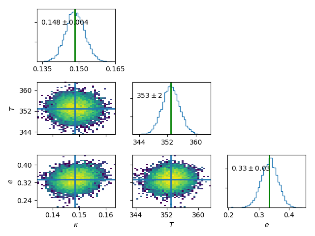
Analysis of a binary system using radial velocity measurement
The radial velocity of a star of mass \(M\) in a binary system with companion of mass \(m\) in an orbit with time period \(T\) and eccentricity \(e\) is given by
The true anomaly \(f\) is a function of time, but depends upon \(e\), \(T\), and \(\tau\) via,
The actual radial velocity data will differ from the perfect relationship given above due to the observational uncertainty (variance \(\sigma_v^2\)) and intrinsic variability of a star (variance \(S^2\)) and we can model this by a Gaussian function \(\mathcal{N}(.|v,\sigma_v^2+S^2)\). For radial velocity data \(D\) defined as a set of radial velocities \(\{v_1,...,v_M\}\) at various times \(\{t_1,...,t_M\}\), one can fit and constrain seven parameters, \(\theta=(v_{0}, \kappa, T, e, \tau, \omega, S)\), using the Bayes theorem as shown below
We implement this as shown below.
# functions for computing the radial velocity curve
def true_anomaly(t,tp,e,tau):
   temp1=np.min((t-tau)/tp)-1
   temp2=np.max((t-tau)/tp)+1
   u1=np.linspace(2*np.pi*temp1,2*np.pi*temp2,1000)
   ma=u1-e*np.sin(u1)
   myfunc=scipy.interpolate.interp1d(ma,u1)
   u=myfunc((2*np.pi)*(t-tau)/tp)
   return 2*np.arctan(np.sqrt((1+e)/(1-e))*np.tan(0.5*u))

def kappa(t,e,m,mc,i):
   au_yr=4.74057 # km/s
   G=4*np.pi*np.pi*np.power(au_yr,3.0) # [km/s]^{3}*[yr]^{-1}*[M_sol]
   nr=np.power(2*np.pi*G,1/3.0)*mc*np.sin(np.radians(i))
   dr=np.power(t/365.0,1/3.0)*np.power(m+mc,1/3.0)*np.sqrt(1-e*e)
   return nr/dr

def vr(t,kappa,tp,e,tau,omega,v0):
   omega=np.radians(omega)
   f=true_anomaly(t,tp,e,tau)
   return kappa*(np.cos(f+omega)+e*np.cos(omega))+v0

# model for describing a binary system
class binary_model(bmcmc.Model):
   def set_descr(self):
       # setup descriptor
       self.descr['kappa']     =['p',0.1,0.1,r'$\kappa$ ',1e-10,10.0]
       self.descr['tp']  =['p',365.0,10.0,r'$T$ ',1e-10,1e6]
       self.descr['e']      =['p',0.5,0.1,r'$e$ ',0,1.0]
       self.descr['tau']     =['p',50.0,10.0,r'$\tau$ ',-360.0,360.0]
       self.descr['omega']=['p',180.0,10.0,r'$\omega$ ',-360,360.0]
       self.descr['v0']=['p',0.0,1.0,r'$v_0$ ',-1e3,1e3]
       self.descr['s']=['p',0.02,1.0,r'$\sigma$ ',1e-10,1e3]

   def set_args(self):
       # setup data points
       np.random.seed(17)
       kappa=0.15
       tp=350.0
       e=0.3
       tau=87.5
       omega=-90.0
       v0=0.0
       print tau,omega

       self.args['t']=np.linspace(0,self.args['tp']*1.5,self.eargs['dsize'])
       vr1=vr(self.args['t'],kappa,tp,e,tau,omega,v0)
       self.args['vr']=vr1+np.random.normal(0.0,self.args['s'],size=self.eargs['dsize'])


   def lnfunc(self,args):
       vr1=vr(args['t'],args['kappa'],args['tp'],args['e'],args['tau'],args['omega'],args['v0'])
       temp=-np.square(args['vr']-vr1)/(2*args['s']*args['s'])-np.log(np.sqrt(2*np.pi)*args['s'])
       return temp
Create an object of the model.
>>> m1=binary_model(eargs={'dsize':50})
Run the sampler.
>>> m1.sample(['kappa','tp','e','tau','omega','v0'],50000,ptime=10000)
Plot the results.
>>> plt.figure()
>>> m1.plot(keys=['kappa','tp','e'],burn=10000)
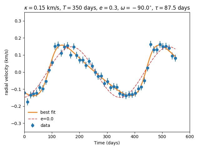
Plot the best fit model.
res=m1.best_fit()
args=m1.args
t=np.linspace(0,np.max(m1.args['t']),1000)
plt.figure()
plt.errorbar(args['t'],args['vr'],yerr=args['s'],fmt='o',label='data')
plt.plot(t,vr(t,res[0],res[1],res[2],res[3],res[4],res[5]),label='best fit',lw=2.0)
plt.plot(t,vr(t,res[0],res[1],0.0,res[3],res[4],res[5]),'r--',label='e=0.0',lw=1.0)
plt.title(r'$\kappa=0.15$ km/s, $T=350$ days, $e=0.3$, $\omega=-90.0^{\circ}$, $\tau=87.5$ days')
plt.xlabel('Time (days)')
plt.ylabel('radial velocity (km/s)')
plt.legend(loc='lower left',frameon=False)
plt.axis([0,600,-0.35,0.35])
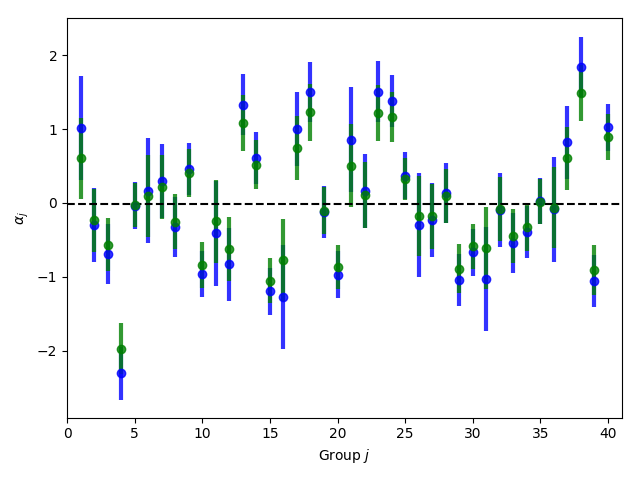
Group means
Given data \(Y=\{y_{ij}|0<j<J,o<i<n_j\}\) grouped into \(J\) independent groups, we want to find the group mean \(\alpha_j\) and the distribution of group means modelled as \(\mathcal{N}(\alpha|\mu,\omega^2)\). The posterior we wish to sample is
class gmean(bmcmc.Model):
  def set_descr(self):
      # Setup descriptor.
      self.descr['alpha']   =['l1',0.0,1.0,r'$\alpha$',-1e10,1e10]
      self.descr['mu']      =['l0',1.0,1.0,r'$\mu$'   ,-1e10,1e10]
      self.descr['omega']   =['l0',1.0,1.0,r'$\omega$',1e-10,1e10]

  def set_args(self):
      # Create data points.
      np.random.seed(11)
      self.eargs['mu']=0.0
      self.eargs['omega']=1.0
      self.eargs['sigma']=1.0

      self.data={}
      self.data['y']=[]
      self.data['gsize']=np.array([2,4,6,8,10]*(self.eargs['dsize']/5))
      self.data['gmean']=np.random.normal(self.eargs['mu'],self.eargs['omega'],size=self.data['gsize'].size)
      for i in range(self.data['gsize'].size):
          self.data['y'].append(np.random.normal(self.data['gmean'][i],self.eargs['sigma'],size=self.data['gsize'][i]))

  def lnfunc(self,args):
     # log posterior
      temp1=[]
      for i,y in enumerate(self.data['y']):
          temp1.append(np.sum(self.lngauss(y-args['alpha'][i],self.eargs['sigma'])))
      temp1=np.array(temp1)
      temp2=scipy.stats.norm.logpdf(args['alpha'],loc=args['mu'],scale=args['omega'])
      return temp1+temp2

  def myplot(self):
      # Plot the results
      plt.clf()
      burn=1000
      x=np.arange(self.eargs['dsize'])+1
      stats=[[],[]]
      for i,y in enumerate(self.data['y']):
          stats[0].append(np.mean(y))
          stats[1].append(self.eargs['sigma']/np.sqrt(y.size))
      plt.errorbar(x,stats[0],yerr=stats[1],fmt='.b',lw=3,ms=12,alpha=0.8)
      plt.errorbar(x,self.mu['alpha'],yerr=self.sigma['alpha'],fmt='.g',lw=3,ms=12,alpha=0.8)

      temp1=np.mean(self.chain['mu'][burn:])
      plt.plot([0,self.eargs['dsize']+1],[temp1,temp1],'k--')
      plt.xlim([0,self.eargs['dsize']+1])
      plt.ylabel(r'$\alpha_j$')
      plt.xlabel(r'Group $j$')
Run and plot
>>> m1=gmean(eargs={'dsize':40})
>>> m1.sample(['mu','omega','alpha'],10000)
>>> m1.myplot()
Extra details
To better understand as to how the code works, it is
instructive to look at the __init__ method of bmcmc.Model. It
creates the dictionaries self.descr and self.args so
the user does not have to create them. It then
calls self.set_descr(). After this it initializes all level-0 parameters
in self.args to values from self.descr. So
parameters of the model that are to be kept free do not need to be
initialized. The user can reinitialize them
set_args which is called next.
If self.eargs['dsize'] , which is the number
of data points, has not been set earlier, it must be
specified in set_args. Any level-1 parameter that
is not initialized in set_args, is done using values
from self.descr.
def __init__(self,eargs=None):
    self.eargs=eargs
    self.args={}
    self.descr={}
    self.set_descr()
    for name in self.descr.keys():
        if (self.descr[name][0]=='l0'):
            self.args[name]=np.float64(self.descr[name][1])
    self.set_args()
    for name in self.descr.keys():
        if (self.descr[name][0]=='l1'):
            if name not in self.args.keys():
                self.args[name]=np.zeros(self.eargs['dsize'],dtype=np.float64)+self.descr[name][1]